阅读量:

电影评论分类：二分类问题

简介

本例出自《Python 深度学习》，自己做了一个简单的总结归纳。

完整代码请参考：https://github.com/fchollet/deep-learning-with-python-notebooks

主要流程

数据预处理

graph LR
    A[原始评论] --> |关键词分割|C[建立关键词索引]
    C --> |将关键词转索引|D[原始评论转向量]
    D --> 列表编码为二进制矩阵

graph LR
    原始评论标签 --> 二制化标签

训练模型

graph LR
    A1(第一层:16个输出单元) --> A[构建模型]
    A2(第二层:16个输出单元) --> A
    A3(第三层:1个输出单元) --> A
    A ==> B[编译模型]
    B1(配置优化器和损失函数) --> B
    B ==> C[加入验证集训练模型]
    C ==> D[绘制图表观察模型最佳参数]
    D1[欠拟合与过拟合之间] --> D
    D ==> E[选择最佳参数训练模型]
    E ==> F[在新数据上使用模型]

代码

加载数据集

注意：第一次加载会下载文件，速度较慢

from keras.datasets import imdb

# 加载 IMDB 数据集
(train_data, train_labels), (test_data, test_labels) = imdb.load_data(num_words=10000)  # 取一万个词

整数序列转二进制矩阵

import numpy as np

# 将整数序列编码为二进制矩阵
def vectorize_sequences(sequences, dimension=10000):
    print((len(sequences), dimension))
    results = np.zeros((len(sequences), dimension))
    for i, sequence in enumerate(sequences):
        results[i, sequence] = 1.
    return results

x_train = vectorize_sequences(train_data)
x_test = vectorize_sequences(test_data)

向量标签化

# 标签向量化
y_train = np.asarray(train_labels).astype('float32')  # int64转float32
y_test = np.asarray(test_labels).astype('float32')

构建模型

# 构建网络
from keras import layers
from keras import models

model = models.Sequential()
# 第一层，16个隐藏单元，激活函数为relu
model.add(layers.Dense(16, activation='relu', input_shape=(10000, )))
# 第二层，16个隐藏单元，激活函数为relu
model.add((layers.Dense(16, activation='relu')))
# 第三层，输出一个标量（预测结果），激活函数为sigmoid
model.add(layers.Dense(1, activation='sigmoid'))

编译模型

# 编译模型
# 优化器：rmsprop
# 损失函数：binary_crossentropy（仅包含一个单元的模型可以采用，替代方案：mean_squared_error）
# 指标：精确
model.compile(optimizer='rmsprop', loss='binary_crossentropy', metrics=['accuracy'])

加入验证集训练模型

# 留出验证集
x_val = x_train[:10000]
partial_x_train = x_train[10000:]

y_val = y_train[:10000]
partial_y_train = y_train[10000:]

# 训练模型
history = model.fit(partial_x_train, partial_y_train, epochs=20, batch_size=512, validation_data=(x_val, y_val))

绘制图表观察训练过程

history_dict = history.history
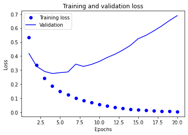
# 绘制训练损失和验证损失
import matplotlib.pyplot as plt


loss = history.history['loss']
val_loss = history.history['val_loss']

epochs = range(1, len(loss) + 1)

plt.plot(epochs, loss, 'bo', label='Training loss')
plt.plot(epochs, val_loss, 'b', label='Validation')
plt.title('Training and validation loss')
plt.xlabel('Epochs')
plt.ylabel('Loss')
plt.legend()

plt.show()

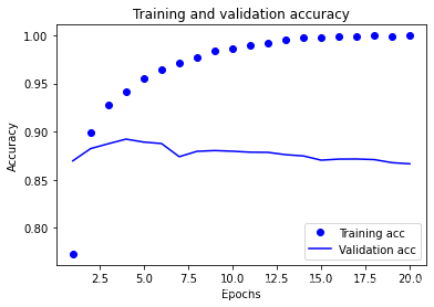
# 绘制训练精度和验证精度
plt.clf()  # 清空图像

acc = history.history['accuracy']
val_acc = history.history['val_accuracy']

plt.plot(epochs, acc, 'bo', label='Training acc')
plt.plot(epochs, val_acc, 'b', label='Validation acc')
plt.title('Training and validation accuracy')
plt.xlabel('Epochs')
plt.ylabel('Accuracy')
plt.legend()

plt.show()

训练模型

# 通过上面的图表发现模型在第四轮之后出现过拟合现象，因此我们选择训练轮数为4
model.fit(x_train, y_train, epochs=4, batch_size=512)

对新数据进行预测

result = model.predict(x_test)
# [0.2930210903453827, 0.8831999897956848]

绘制图表

训练损失和验证损失

# 绘制训练损失和验证损失
import matplotlib.pyplot as plt


loss = history.history['loss']
val_loss = history.history['val_loss']

epochs = range(1, len(loss) + 1)

plt.plot(epochs, loss, 'bo', label='Training loss')
plt.plot(epochs, val_loss, 'b', label='Validation')
plt.title('Training and validation loss')
plt.xlabel('Epochs')
plt.ylabel('Loss')
plt.legend()

plt.show()

训练精度和验证精度

# 绘制训练精度和验证精度
plt.clf()  # 清空图像

acc = history.history['binary_accuracy']
val_acc = history.history['val_binary_accuracy']

plt.plot(epochs, acc, 'bo', label='Training acc')
plt.plot(epochs, val_acc, 'b', label='Validation acc')
plt.title('Training and validation accuracy')
plt.xlabel('Epochs')
plt.ylabel('Accuracy')
plt.legend()

plt.show()

总结

• 通常需要对原始数据进行大量预处理，以便将其转换为张量输入到神经网络中。单词序列可以编码为二进制向量，但也有其他编码方式。
• 带有relu激活的Dense层堆叠，可以解决很多种问题（包括情感分类），你可能会经常用到这种模型。
• 对于二分类问题（两个输出类别），网络的最后一层应该是只有一个单元并使用sigmoid激活的Dense层，网络输出应该是0~1范围内的标量，表示概率值。
• 对于二分类问题的sigmoid标量输出，你应该使用binary_crossentropy损失函数。
• 无论你的问题是什么，rmsprop优化器通常都是足够好的选择。这一点你无须担心。
• 随着神经网络在训练数据上的表现越来越好，模型最终会过拟合，并在前所未见的数据上得到越来越差的结果。一定要一直监控模型在训练集之外的数据上的性能。

评论